R 기초

Data Types

# Character strings
class('abc'); class("TRUE")

# Numeric
class(Inf); class(1); class(-3)

# Logical
class(TRUE); class(FALSE)

# Special values
sqrt(-3)      # NaN: Not a Number
class(NA)     # NA: Missing value
class(NULL)   # NULL: No memory allocated

Variable Assignment

string1 <- 'abc'      # Standard assignment
"data" -> string2     # Rightward assignment
number1 <<- 15        # Global assignment
Inf ->> number2       # Global rightward assignment
logical = NA          # Assign NA to logical variable

Comparison & Logical Operators

string1 == 'abc'
string1 != 'abcd'
string2 > 'DATA'
number1 <= 15
is.na(logical)
is.null(NULL)

!TRUE
TRUE & FALSE
TRUE | FALSE
!(TRUE & FALSE)

Vectors

v4 <- c(3, TRUE, FALSE)   # Coerced to numeric
v5 <- c('a', 1, TRUE)     # Coerced to character
v1 <- c(1:6)

Matrices & Arrays

m1 <- matrix(c(1:6), nrow=2)
m2 <- matrix(c(1:6), ncol=2)
m3 <- matrix(c(1:6), nrow=2, byrow=TRUE)

v1 <- c(1:6)
dim(v1) <- c(2,3)  # Reshape into matrix

a1 <- array(1:12, dim=c(2,3,2))

Lists

L <- list()
L[[1]] <- 5
L[[2]] <- c(1:6)
L[[3]] <- matrix(1:6, nrow=2)
L[[4]] <- array(1:12, dim=c(2,3,2))

Data Frames

v1 <- c(1,2,3)
v2 <- c('a', 'b', 'c')
df1 <- data.frame(v1, v2)

String Manipulation

data <- 'This is a pen'
tolower(data)
toupper(data)
nchar(data)
substr(data, 9, 13)
strsplit(data, 'is')
grepl('pen', data)
gsub('pen', 'banana', data)

Statistical Functions

Function	Description	Example	Output (for `x <- c(2, 4, 6, 8, 10, 12)`)
`mean(x)`	Returns the arithmetic mean (average)	`mean(x)`	`7`
`median(x)`	Returns the median (middle value)	`median(x)`	`7`
`sum(x)`	Returns the total sum of all elements	`sum(x)`	`42`
`max(x)`	Returns the largest value	`max(x)`	`12`
`min(x)`	Returns the smallest value	`min(x)`	`2`
`range(x)`	Returns a vector with the min and max values	`range(x)`	`2 12`
`var(x)`	Returns the sample variance	`var(x)`	`14.4`
`sd(x)`	Returns the sample standard deviation	`sd(x)`	`3.7947`
`which.max(x)`	Returns the index of the first maximum value	`which.max(x)`	`6`
`which.min(x)`	Returns the index of the first minimum value	`which.min(x)`	`1`
`summary(x)`	Returns min, 1st Qu., median, mean, 3rd Qu., and max	`summary(x)`	`Min. 2, 1st Qu. 4.5, Median 7, Mean 7, 3rd Qu. 9.5, Max. 12`
`quantile(x)`	Returns the percentiles/quantiles	`quantile(x)`	`0%: 2, 25%: 4.5, 50%: 7, 75%: 9.5, 100%: 12`

v1 <- seq(2, 12, by=2)
sum(v1)
mean(v1)
median(v1)
var(v1)
sd(v1)
max(v1)
min(v1)
range(v1)
summary(v1)

Skewness & Kurtosis

install.packages("fBasics")
library(fBasics)
skewness(v1)    # Skewness: asymmetry of distribution
kurtosis(v1)    # Kurtosis: peakedness

Data Handling

m1 <- matrix(1:6, nrow=2)
colnames(m1) <- c('c1', 'c2', 'c3')
rownames(m1) <- c('r1', 'r2')

df1 <- data.frame(x=c(1,2,3), y=c(4,5,6))
colnames(df1) <- c('c1', 'c2')
rownames(df1) <- c('r1', 'r2', 'r3')

df1$v1; df1$v2[3]
df1[2,]

Control Structures

# For loop
for(i in 1:3) print(i)

# While loop
i <- 0
while(i < 5) {
  print(i)
  i <- i + 1
}

# If-Else
number <- 7
if(number < 5) {
  print('Less than 5')
} else if(number > 5) {
  print('Greater than 5')
} else {
  print('Equals 5')
}

Functions

comparedTo5 <- function(number) {
  if(number < 5) print('Less than 5')
  else if(number > 5) print('Greater than 5')
  else print('Equals 5')
}

comparedTo5(10); comparedTo5(3); comparedTo5(5)

Apply & Preprocessing

x <- 1:12
head(x, 5); tail(x, 5); quantile(x)

df1 <- data.frame(x=c(1,1,1,2,2), y=c(2,3,4,3,3))
df2 <- data.frame(x=c(1,2,3,4), z=c(5,6,7,8))

subset(df1, x==1)
merge(df1, df2, by='x')

apply(df1, 1, sum)  # row-wise
apply(df1, 2, sum)  # column-wise

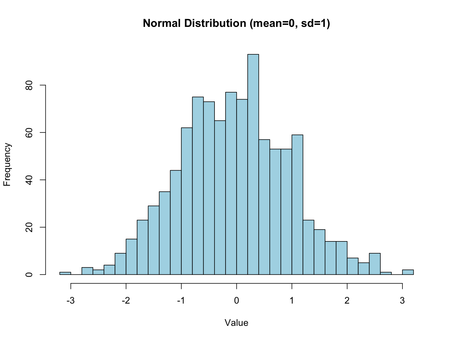
R Functions for Normal Distribution

The normal distribution (also called Gaussian distribution) is a continuous probability distribution that is symmetric around the mean. It is commonly used in statistics and data analysis to model naturally occurring data.

Characteristics of the Normal Distribution

Bell-shaped curve: Symmetrical around the mean.
Mean = Median = Mode
Defined by two parameters: mean (μ), standard deviation (σ)

Function	Description	Example	Output / Note
`dnorm(x)`	Probability density function	`dnorm(0)`	Density at x = 0 (default mean = 0, sd = 1)
`pnorm(q)`	Cumulative distribution function (P(X ≤ q))	`pnorm(1.96)`	≈ 0.975
`qnorm(p)`	Quantile function (inverse of pnorm)	`qnorm(0.975)`	≈ 1.96
`rnorm(n)`	Random generation from normal distribution	`rnorm(5, mean=10, sd=2)`	5 values from N(10, 2²)

# Generate 1000 random values from N(0,1)
data <- rnorm(1000, mean = 0, sd = 1)

# Plot histogram
hist(data, breaks=30, col="lightblue", main="Normal Distribution (mean=0, sd=1)", xlab="Value")

Rplot01

Date & Time

Sys.Date(); Sys.time()
as.Date("2020-01-01")
format(Sys.Date(), '%Y/%m/%d')
format(Sys.Date(), '%A')

unclass(Sys.time())
as.POSIXct(1743844791, origin='1970-01-01')

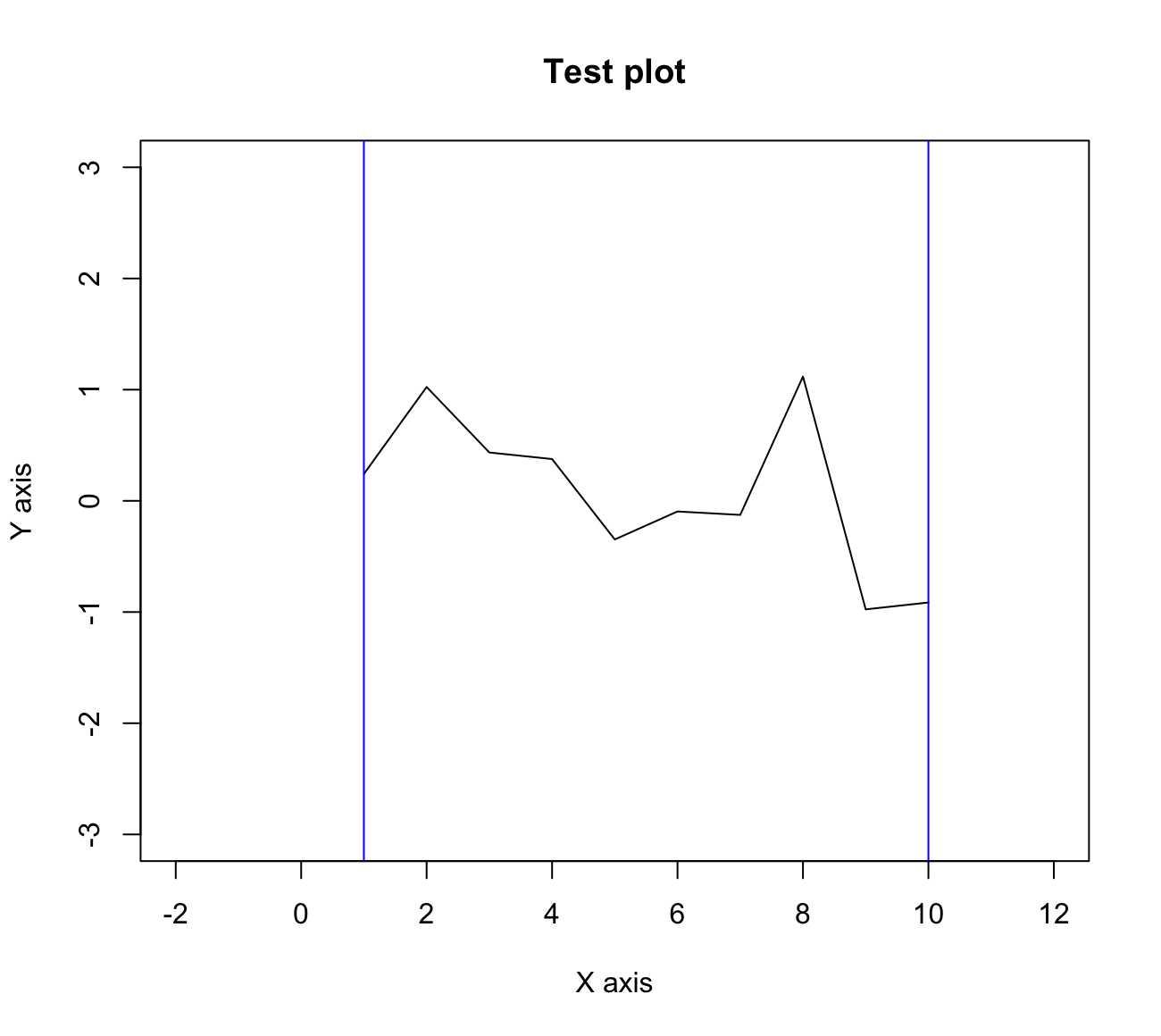
Basic Plotting

x <- 1:10
y <- rnorm(10)

plot(x, y, type='l', xlim=c(-2,12), ylim=c(-3,3),
     xlab='X axis', ylab='Y axis', main='Test plot')

abline(v=c(1,10), col='blue')

R plot

This comprehensive summary is ideal for beginners in R and those reviewing fundamentals in preparation for data science applications. You can reuse these code blocks for projects, notebooks, or presentations.

제1장 R 기초와 데이터 마트

목차